Writing a GPU-Accelerated Path Tracer in Rust - Part 1

Well, it’s that time again. This is the start of a second series of articles on raytracing in Rust following on from my previous series. This time, I’ll be doing all of the rendering on a GPU using Accel - see my previous post on Accel. I thought this would be a good project for learning about GPU programming, see.

Second, this time I want to write a path tracer, rather than a raytracer.

You don’t need to know anything about GPU programming to follow along - I’ll explain things as needed. If you intend to run your code on the GPU though, you should read that post about Accel. As before, I will assume that you’re familiar with the basics of linear algebra (you should know about vectors and matrices, as well as what the dot and cross products are). I’ll also assume that you’ve read the previous series.

Path Tracing

A path tracer is like a raytracer in that it traces rays of light backwards from the camera through a scene. Unlike a raytracer, however, a path tracer traces many rays - often thousands - for each pixel. The rays are scattered randomly off of the objects until they reach a light source, leave the scene entirely, or end for some other reason (eg. reaching a fixed bounce limit). Each ray is colored according to the objects it bounced off of and the light source it reached, and the final color of a pixel is the average of all rays traced through it.

This more-accurately reflects the behavior of real light; what our eyes see is the sum total of all light received from a point in the world; those photons took many different paths and were colored by many different objects on their way to that point. For example, when a bright red object is in bright light it makes nearby objects appear to glow red with reflected light. When a sunbeam shines through a glass object, you can see a pattern of light and dark where the object focuses some of the light (these patterns are called ‘caustics’). Path tracing makes it easy to render these effects where ray tracing does not.

That randomness has a downside as well - it can produce very noisy images if not enough paths are traced per pixel. We say that the image has converged when there are enough paths to remove visible noise. Additionally, tracing hundreds or thousands of rays per pixel takes much more computation than tracing one, so, all else being equal, path tracers take longer to render an image. Caustics in particular only show up if the scattered rays take very precise paths and so are even noisier than the rest of the scene. More advanced algorithms like Bi-Directional Path Tracing speed up rendering times by making the image converge with fewer paths, especially when rendering special effects like caustics. I’ll just be implementing the basic path tracing algorithm here though.

Basics of GPU Acceleration

Raytracing is a good problem for GPU acceleration because it’s massively parallel - every pixel (or in a path tracer, potentially every ray), can be computed in parallel with every other pixel. GPUs are fast because they can efficiently run thousands of parallel threads. Even though each individual thread is significantly slower than a CPU thread, working together they can do a lot of work quickly.

It’s not necessary to know a whole lot about GPU acceleration for this series. I will mostly ignore efficiency in this post; I’ll make it work, then make it fast later on. I’ll explain more about how to write efficient GPU code if and when it becomes relevant.

Setting the Scene

My raytracer only handled spheres and planes. I was bored with that, so the path tracer will work with polygon meshes instead. Crates.io already has a Wavefront OBJ parsing library. Polygons in the OBJ format consist of a list of indexes into a position array. I expanded that into a structure where each polygon contains three 3D vectors representing the vertices. I made this choice on the basis that this is easier to work with, but it also avoids the indirection of looking up the vertex index, then looking up the vertex. This structure is quite inefficient, but it’s good enough for now. I may opt to rework this later.

My meshes only contain triangles but some have quads or even more complex polygons. We’ll convert those polygons to triangles for simplicity. To do this, take the first vertex then iterate over the remaining vertices using a two-element sliding window. This produces a series of three-vertex triangles. See the following pseudocode:

vertex1 = polygon[0]
for (int k = 1; k < polygon.length - 1; k++) {
    vertex2 = polygon[k]
    vertex3 = polygon[k+1]
    add_triangle(vertex1, vertex2, vertex3)
}

Now that we have triangles, we need rays and a way to intersect those rays against the triangles. To start with, we only need prime rays (the initial rays traced from the camera out). I just copied the prime-ray generation code from the old raytracer. This is an advantage to writing the path tracer in pure Rust rather than CUDA C - I can reuse existing Rust code without needing to rewrite it.

Ray-Triangle Intersection Test

The nice thing about triangles is that all points lie in the same plane. This is helpful for the intersection test, since we can break it into two tests - does the ray intersect the plane, and if so, does it intersect the plane inside the triangle?

First, we calculate the normal of the plane. Recall that the cross product of two vectors produces a new vector perpendicular to both. To generate the normal of a plane we take the cross product of two vectors which lie in that plane. We can generate two vectors in the plane of the triangle by subtracting the vertices from each other:

let a = v1 - v0;
let b = v2 - v0;

let normal = a.cross(b).normalize();

This will result in one of two vectors depending on the order of the vertices. This makes sense; a plane has two sides and therefore two opposing normal vectors. Which one we see depends on whether the vertices were stored in clockwise or counterclockwise order. Correct OBJ files are always in counterclockwise order and Scratchapixel uses the same convention so we should be OK.

Last time, I passed over explaining how the plane-intersection test works, but I’ll try now. I can’t think of a good intuitive geometric explanation of why this works, so I’ll just explain the math.

Planes are defined by an equation Ax + By + Cz + D = 0. Some sources use Ax + By + Cz = D instead; this is just a different convention. You can convert between the two by negating D, but Scratchapixel uses the former equation so I will as well.

Scratchapixel’s derivation and implementation of this equation (here) is wrong. This confused me for hours until I found another source that derived it correctly. The other source used the other convention, which confused me even more. Eventually I did the derivation myself on paper and spotted the mistake. I’ll give the correct version.

This equation is equivalent to N dot P + D = 0 where N is a normal of the plane (A, B, C), P is any point on the plane (x, y, z), and D is the smallest distance between the plane and the origin. We also have the ray equation Ray(t) = O + tR where O is the origin of the ray, R is the direction, and t is some distance along the direction. If the ray intersects the plane then the intersection point must lie in the plane, so we can substitute Ray(t) for P get the following equation:

N dot Ray(t) + D = 0
N dot (O + tR) + D = 0
N dot O + t(N dot R) + D = 0

// Rearrange to solve for t...
N dot O + t(N dot R) = -D
t(N dot R) = -D - (N dot O)
t = (-D - (N dot O))/(N dot R)

We have N from earlier. O and R are the components of the ray we’re tracing. We need D before we can get t. We can calculate D using N and any point on the plane. The vertices of the triangle are also points on the plane, so plug any vertex (I’ll use the first one) into the equation and solve for D like so:

N dot v0 + D = 0
D = -(N dot v0)

(This is where Scratchapixel goes wrong; they forgot the negative sign)

Thus, we have the pseudocode for the intersection of a ray and a plane:

let D = -(normal.dot(polygon.vertices[0]));
let t = (-D - (normal.dot(ray.origin))/(normal.dot(ray.direction));

// Remove the double-negation of D
let neg_D = normal.dot(polygon.vertices[0]);
let t = (neg_D - (normal.dot(ray.origin))/(normal.dot(ray.direction));

Finally, plug t back into the ray equation to get the intersection point:

let p = ray.origin + t * ray.direction;

There are a few corner cases, however. If the ray is parallel to the triangle, then the dot-product of the normal and the ray direction will be zero - a divide-by-zero error. In that case we know the ray will not intersect the plane at all so we can return no-intersection.

If the distance is negative, this means that the triangle’s plane is behind the origin of the ray, and so it can’t intersect. Again, we check for that and return no-intersection.

Triangle Intersection Part 2

Now that we’ve found the point where the ray intersects the triangle’s plane, we need to check if that point is inside the triangle. First, we define a test to check if a point is on the left side or right side of a vector.

Consider the following image:

We can use the cross product and dot product to determine if the vectors B and B’ are on the left or right side of the vector A. For this example, let’s use the following numbers:

A = (0, 1, 0)
B = (-1, 1, 0)
B' = (1, 1, 0)

Recall that the cross product is defined like so:

C.x = A.y * B.z - A.z * B.y
C.y = A.z * B.x - A.x * B.z
C.z = A.x * B.y - A.y * B.x

We’ll calculate C = A.cross(B) and C' = A.cross(B'). A.z, B.z and B’.z are all zero in this case, so C.x and C’.x will also be zero. The same is true for C.y and C’.y. C.z and C’.z, however…

C.z = 0 * 1 - 1 * -1
    = 0 - (-1)
    = 1

C'.z = 0 * 1 - 1 * 1
     = 0 - 1
     = -1

C = (0, 0, 1) and C’ = (0, 0, -1). Conventionally, negative-Z means “into the screen”, so this means that C points out of the screen while C’ points into it. This gives us our test; B is on the left side of A and so the cross product points out of the screen, where B’ is on the right side of A so the cross product points into the screen. To handle arbitrary planes in 3D space, we can calculate the dot product of C and C’ against the normal vector N. N and C point in the same direction so their dot product will be positive, while N and C’ point in opposite directions, so their dot product will be negative.

Putting that all together, we get our left-side test: left = A.cross(P).dot(N) > 0 where A and P are the vector and point we want to check and N is the surface normal of the plane.

Now that we have that, we can test if a point is inside the triangle. If the point is to the left of all three edges of the triangle (in counter-clockwise order), it’s inside the triangle.

This is an intersection test that we can implement in code. As a side note, this left-of-all-edges test works on all convex polygons, not just triangles.

A Diversion

At this point my path tracer started crashing mysteriously - even forcing a display reset. I suspected a segfault (I’m using raw pointers, so Rust can’t prevent memory errors), but I checked my code and I couldn’t find one. Then I noticed that it worked - but only if I rendered fewer polygons.

After some internet searching, I discovered that most operating systems - including Linux and Windows - have a watchdog timer. If the GPU is busy and unable to repaint the screen for more than a few seconds, the OS resets it, killing the misbehaving kernel. There are ways around this (at least on Windows) by changing registry settings. Some graphics cards can be set into a different mode where it isn’t available for painting the screen, but I only have the one GPU, so that doesn’t work for me. For now, I’ll break up the image into smaller blocks so that the card can render each block inside the time limit, and as my code grows more complex I will edit the registry to increase the time limit.

First Image

Whew! After all of that, I threw together some basic code to render an image. It’s simple code for now; it traces one ray for each pixel and sets the color to bright green if it hits a polygon.

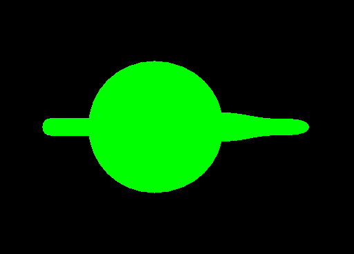
What’s that Pokemon object? The Utah Teapot as seen from above!

Positioning

Using triangle meshes raises another consideration. We defined spheres with a center point and size; for planes we provided a point and a normal vector. How do we place a mesh within the scene? We can move a mesh by adding a constant to each component of each vertex - but how do we scale or rotate a mesh? We use matrices - specifically, 4x3 (or sometimes 4x4) matrices.

This article is getting quite long already, so I’ll just lay down some basics (again, assuming that you know what matrices and vectors are). It’s easiest to describe this in software terms, so think of a 4x3 matrix as a function which takes a 3D vector and returns a transformed 3D vector. I won’t go into too much detail (see links below for that), but it’s possible to construct a matrix that performs the translation function - ie. it adds a value to each component of the vector. Likewise, there are matrices that will scale a vector or rotate it around the X/Y/Z axes.

Those familiar with functional programming will know how you can package up a function, pass it around, combine it with other functions and ultimately apply it to some input to get some output. The same is true for these function-matrices (or really, any matrix). We apply a matrix to a vector by computing the matrix-vector multiplication, which produces a new vector. We can compose function matrices by multiplying the two matrices together to produce a new matrix which performs the function of both.

To position an object in the world we construct a matrix/function that converts the vertex positions of the input object to some new vertex positions representing where we want the object to be in the world. More formally, this matrix converts from the object’s coordinate space to the world’s coordinate space - and this is why these matrices are typically called object-to-world matrices. Once we define the object-to-world matrix, we can apply it to (multiply it with) the vectors that make up the polygons of the object, producing new vertices which position the polygons in the right place in the world.

Now, you could write the object-to-world matrix by hand, but just as with software it’s easier to define building-blocks (eg. code to create translation or scaling matrices). We can then compose the functions together - for example, scale by ³⁄₅, then rotate about the X axis by 90 degrees, then translate down by one unit - to get the object-to-world matrix.

Just like with function composition, it’s important to be aware of the order in which the functions will be applied - f(g(x)) is not necessary the same as g(f(x)), and translate(0.0, 0.0, 1.0).multiply(scale(0.6)) is not the same as scale(0.6).multiply(translate(0.0, 0.0, 1.0). Depending on how you implement your matrix-multiply function, the function composition might go right-to-left (ie. the right-most operation is applied first) or left-to-right. It’s important to know which one you’re using when you construct the object-to-world matrix. This matrix-multiply code makes it so that matrices compose right-to-left, which is the normal convention:

We then multiply the matrix against every vertex of every triangle and collect the new vectors into new triangles which represent the new position of the object in the world. As a side note - I didn’t cover this in my last series (and it won’t be needed in this one either) but you can use this technique to position the camera in the world as well. Apply the matrix to the origin and direction of the prime rays. Be aware that applying a matrix to a point in space is not the same as applying it to a direction vector - see the links below for more detail.

If you’re interested in the theory behind this, I recommend 3Blue1Brown’s excellent series on linear algebra. It covers the concept of matrices-as-functions with more depth and clarity than I could manage. Also check out Scratchapixel’s articles on Geometry, which I used when I wrote this matrix-math code for my last raytracer.

Conclusion

We have some building blocks and a rudimentary GPU-accelerated raytracer. As usual, check out the code on GitHub and stay tuned for the next post, where we’ll turn this into a true path-tracer and add support for refractive and reflective surfaces.

Thanks to Daniel Hogan for beta-reading this article and offering helpful comments.