Hello, and welcome to part two of my series on writing a GPU-accelerated path tracer in Rust. I’d meant to have this post up sooner, but nothing ruins my productivity quite like Games Done Quick. I’m back now, though, so it’s time to turn the GPU ray-tracer from the last post into a real path tracer.
Tracing Paths
As mentioned last time, Path Tracing is an extension to Ray Tracing which attempts to simulate global illumination. That is, the light that you see from objects or areas that don’t have a direct path to light sources. If you look around, you can probably find places which are shaded from all local light sources and yet are not completely dark. This is because some light is being scattered off other objects, lighting up the dark corners and then reaching your eyes.
Path tracing attempts to simulate this by tracing a complete path from the camera back to a light source, scattering randomly off of objects in the way. In reality, there are infinitely many different paths a photon might have taken to reach your eyes, and it may have bounced arbitrarily many times. Our computing power is unfortunately finite, so we need to find ways to cheat. We can make this problem manageable using a technique called Monte Carlo Integration. You can look that up in more detail if you want to. For our purposes this means that we take a random sample of the problem (ie. a number of random paths through the scene) and compute the average brightness.
As you might imagine, the random nature of this causes visual noise to appear in the final image. We’ll deal with this by ignoring it, and just cranking up the number of paths we trace per pixel - this will decrease the noise but not eliminate it. Real path tracers use more-advanced algorithms which produce less noise for a given number of paths and sometimes perform a de-noising operation after rendering as well. I have no idea how that works. Maybe I’ll take the time to learn someday!
We can further simplify matters by using the path-tracing algorithm to do all of our lighting calculations, rather than tracing shadow rays like we did in the original raytracer series. A production-quality renderer would probably use the global illumination as just a part of the lighting equation, but it’s good enough for us all by itself.
Additionally, we’ll cut off paths after a fixed number of bounces. In practice, most photons lose almost all of their energy after a few bounces anyway, so they can mostly be ignored without a major effect on the resulting image. This does bias the results a bit, making the image darker than it really should be, but hopefully not enough to be noticeable.
On Surfaces
It’s easy enough to bounce rays off of polished glass or metal surfaces. We implemented that in the previous series on raytracing, and it’s no different now. For these surfaces, there’s a single deterministic direction for the new ray, based on the surface normal and the incident ray.
Matte surfaces (also known as diffuse surfaces) are different, however. They scatter incident light randomly over a half-sphere above the point of contact, centered on the surface normal. To simulate this, we’ll have to generate random numbers on the GPU. Ideally, they should be very cheap to generate but still have good-quality pseudorandomness. Then, we need to use those random numbers to choose a direction vector in the appropriate half-sphere. First, let’s look at selecting a direction for the bounce ray; I’ll come back to generating random numbers later.
Hemispheres
At a high level, selecting a random direction goes like this. Suppose you wanted to pick a random spot in the sky to point a telescope at. You might do this by generating one random number to indicate which direction you should face (eg. zero to two*PI radians from north) and one number to indicate how high you should look (ranging from zero at the horizon to PI/2 radians, or straight up). These two numbers are called the azimuth (direction angle) and elevation (angle up into the sky), and together they’re called polar coordinates. Then we need to convert these two coordinates into the Cartesian system used by our other code.
Normally, converting polar coordinates to cartesian would be done with the following equations:
// r here is the radius of the sphere, which in our case is always 1
// so I'll ignore it from now on.
azimuth = rand() * PI * 2
elevation = rand() * PI / 2
x = r * sin(elevation) * cos(azimuth)
y = r * cos(elevation)
z = r * sin(elevation) * sin(azimuth)
For efficiency, it would be nice if we could avoid computing so many trigonometric functions. They tend to be slow at the best of times. What’s worse is that I had to use software implementations of these functions because I couldn’t figure out how to get rustc to generate the appropriate sin/cos/tan PTX instructions, so they’re even slower on the GPU.
Instead, we can generate a random number for cos(elevation) directly, and then calculate
sin(elevation) from that.
// We have the following rule from trigonometry:
sin^2(angle) + cos^2(angle) = 1

// Move the cos term to the other side of the equals
sin^2(angle) = 1 - cos^2(angle)

// Take the square root
sin(angle) = sqrt(1 - cos^2(angle))

// cos^2(angle) = cos(angle)^2, and we already have cos(angle), so...
y = rand()
sin(angle) = sqrt(1 - y * y);
This gives us a faster way to generate a point on a hemisphere:
azimuth = rand() * PI * 2
y = rand()
sin_elevation = sqrt(1 - y * y)
x = sin_elevation * cos(azimuth);
z = sin_elevation * sin(azimuth);
Now we only have to compute two slow trigonometric functions instead of four.
Technically, this is not just an optimization. This is known as Cosine-weighted Importance Sampling and apparently it has some nice statistical properties which reduce the noise in the final image. I’m afraid I don’t really know the details and couldn’t find a good explanation - if you know of one then please send me a link.
This code generates vectors in a hemisphere centered on the Y axis above the origin. We want them to be centered on the surface normal above the intersection point. We can do this by defining a new coordinate system using the surface normal as our ‘Y-axis’ and creating other vectors to serve as X and Z axes. Then we can transform our hemisphere-vector into this new coordinate system.
The Y axis of our temporary coordinate system is given - it’s the surface normal. How do we generate the other vectors? We really only need one vector perpendicular to the surface normal. If we have that, we can generate the third using the cross product.
First, lets return to the plane equation from last time:
Ax + By + Cz + D = 0
// Alternately, we could use the coordinates of our hit normal N.
N.x * x + N.y * y + N.z * z + D = 0
In this case, we don’t care about D so we’ll just ignore it. Additionally, in this case we’re interested in a plane that is perpendicular to the hit normal (our Y axis) and so every point on that plane will have a Y coordinate of zero, so we can ignore that as well.
N.x * x + N.z * z = 0
N.x * x = -(N.z * z)
Now, consider - which values of x and z could make this equation true (remember that N.x and N.z are fixed already)? Well, if x = -N.z and z = N.x, that would make both sides equal. Another option would be if z = -N.x and x = N.z. We can use this to generate a perpendicular vector to our hit normal. I admit, I don’t fully get why this works, but it does. I think we just need to find a vector that points to some point on the plane, since any point on the plane creates a vector perpendicular to the hit normal.
let Nt = Vector(N.z, 0, -N.x).normalize();
let Nb = N.cross(Nt);
There is one more wrinkle, though. If N.z and N.x are both close to zero then normalizing (which
involves dividing by sqrt(N.x * N.x + N.z * N.z)) could result in a very long vector, or even a
divide-by-zero. We can avoid this by performing a similar trick using the Y coordinate if that’s
larger than the X coordinate, like so:
if (fabs(N.x) > fabs(N.y)) {
    Nt = Vector(N.z, 0, -N.x).normalize();
}
else {
    Nt = Vector(0, -N.z, N.y).normalize();
}
Nb = N.cross(Nt);
Now we have an X/Y/Z coordinate system comprised of (Nb, N, Nt). To transform our hemisphere vector to this coordinate system, we multiply and sum all of the vectors against the hemisphere vector, like so:
new_ray_direction = Vector(
    hemisphere.x * Nb.x + hemisphere.y * N.x + hemisphere.z * Nt.x,
    hemisphere.x * Nb.y + hemisphere.y * N.y + hemisphere.z * Nt.y,
    hemisphere.x * Nb.z + hemisphere.y * N.z + hemisphere.z * Nt.z,
)
You may notice that this looks a lot like a matrix multiplication. Recall from the previous post how we use matrices to transform vectors into new positions? It’s the same principle here, except that I’ve performed the multiplication directly rather than constructing a matrix object.
Generating Random Floats
Next we need to be able to generate random numbers that we can use in this process. Normally, I
would just use the rand crate, but in this case I can’t. It does have no_std support, but Xargo
needs a target JSON file for every crate and rand doesn’t provide one. I could clone rand
locally and add one, but it’s kind of fun to DIY it. I don’t need a cryptographically-secure RNG to
render pretty pictures, so I’m just going to wing it.
You can use any pseudo-random number generator you like. I’m I’m going with an xorshift generator because it’s small (both in terms of code and memory) and because it’s fast. This generates a 32-bit unsigned integer as output. We need a floating-point value in the range [0.0, 1.0). We could simply divide by the maximum value of a u32. Or, we could do some evil floating-point bit-level hacking to make it go faster. I know which one I’m going with!
Standard (IEEE754) floating-point numbers are made up of a sign bit, some number of exponent bits and the rest are mantissa bits. The sign bit we already know; it should be positive. Think of the exponent bits as selecting a window between two consecutive powers-of-two, and the mantissa bits as selecting an offset within that window (see Floating Point Visually Explained for more details).
Therefore, if we can generate a random mantissa section and set the sign and exponent bits to the right value, we can generate a random float without doing a floating-point division (which is somewhat expensive).
As a side note - this is silly levels of micro-optimization, especially considering that we haven’t even tried to optimize the rendering algorithm yet. I’m just doing this for fun, not because I think the extra performance is actually worth it. Additionally, this algorithm was inspired by this blog post.
Anyway, we know the right window for our numbers - [0.0, 1.0). However, it’s easiest to do this if we select the window of the right width to start with, so I’ll go with generating a number in the range of [1.0, 2.0) and then subtract 1.0 from it afterwards. This also allows us to ignore some extra complexity that comes with values close to zero.
For IEEE single-precision floating points, this gives us a fixed bit pattern for the first 9 bits, followed by 23 random bits. I used a floating-point converter I found on Google to get the correct bit pattern for the sign and exponent bits - 0x3F800000. Then we mask out the lower 23 bits of our random integer (mask is 0x007FFFFF) and combine. Finally, we transmute the resulting bit pattern into a 32-bit float, subtract 1.0 and return.
fn random_float(seed: &mut u32) -> f32 {
    let mut x = *seed;
    x ^= x >> 13;
    x ^= x << 17;
    x ^= x >> 5;
    *seed = x;
    let float_bits = (x & 0x007FFFFF) | 0x3F800000;
    let float: f32 = unsafe { ::core::mem::transmute(float_bits) };
    return float - 1.0;
}
Some quick testing confirms that the output is at least approximately uniform, so it’s probably good enough for our purposes. One neat thing about this trick is that it’s customizable; if you want numbers in the range [-1.0, 1.0) you can use 0x40000000 instead of 0x3F800000 to select the exponent for the [2.0, 4.0) range and then subtract 3.0.
Putting it All Together
Now we can create a random scatter direction, so we can have our backwards light rays bounce realistically when they intersect an object. We need to bounce each ray through the scene, adding the emission of any glowing objects it encounters.
On the CPU, I would do this recursively. I might have a function to trace a ray and return the color of the light coming from that direction, and it would then call itself recursively to some bounce limit. I’d multiply that light by the albedo and color of the object, a factor based on the angle of incidence and maybe a constant fudge factor to make things look nice, and return it.
CUDA code technically can do recursion, but every time I try it causes the kernel launch to fail
with an OUT_OF_RESOURCES error. CUDA’s error messages are super unhelpful, so I have no idea why.
I’ll have to do this with iteration, then. This is a bit tricky to think about because it’s sort of backwards from how I would normally think about light. I keep an accumulator color to hold the color for the path as it’s being traced, and another mask color. The mask color is multiplied by the emission of each intersected object and added to the accumulator. The mask represents the accumulated absorption of all of the objects that the ray has intersected until now.
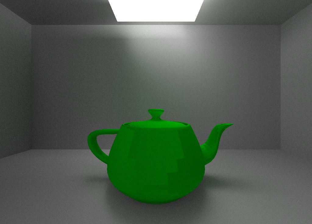
Some examples are in order. If the ray we trace directly intersects a glowing object (0.8, 0.8, 0.8), the mask will be (1.0, 1.0, 1.0), so the glow color of the object will be added directly to the accumulator. If we bounce off a green (0.0, 1.0, 0.0) object first, the mask picks up the green color, and it might be set to (0.0, G, 0.0), where G is < 1.0. Then, when we multiply the mask by the emission of the glowing object on the next intersection, the accumulator is set to (0.0, 0.8 * G, 0.0).
The reason why the mask is less bright than the color of the object has to do with the albedo of the object (how much of the incoming light does it reflect away) and the angle of incidence of that light.
Afterwards, we generate a new random direction for the ray and repeat the process.
Now that we have code to sample the color at a pixel, we need to average the colors together to form a pixel in our resulting image. Since the scattered rays may not ever intersect with a light source, there would be a huge amount of noise in our image if we only sampled each pixel once. Instead, path tracers trace many (hundreds or thousands) of scattered paths through the scene and average all of the resulting samples together.
This raises another problem. Remember the 3-second time limit on kernel execution I mentioned in the last post? There’s no way my card can render a decent-sized image with thousands of paths per pixel in 3 seconds. It can’t even come close to tracing enough rays in one 3-second window to make even a small part of the image converge.
To work around this, I render each block of the image many times, accumulating the results in the image buffer. In this way, I can render an arbitrarily complex scene (within limits, anyway; it has to be able to complete at least one sample for each pixel in time) given enough time.
Currently, this takes hours for a decent-sized image of a not-very-complex scene. There are ways to speed it up, though, and I’ll cover that in the next post.
Reflection and Refraction
The math behind reflective and refractive surfaces is the same for path tracers as it is for raytracers, so I won’t re-tread old ground here. See the previous series for more on that. Instead I’ll cover some of the challenges that I ran into while implementing them in my path tracer.
Reflection is pretty simple; if a surface is reflective we use the code from the last series to generate the bounce direction instead of the random-point-on-hemisphere code. Refraction is more complex to implement though.
See, the iterative path-tracing loop I created above assumes that it’s only ever tracing one ray at a time. This assumption doesn’t work with refraction, though, which requires tracing both a reflection ray and a transmission ray, each containing part of the power of the original ray.
In the old CPU-based raytracer, we could implement this by making another recursive call with the other direction and combining the two colors. As I mentioned earlier though, recursion on the GPU doesn’t seem to work for me, so we have to find a way to do it iteratively.
The normal trick when converting these sorts of recursive algorithms to be iterative is to keep some extra space to store the data that would otherwise be stored in the call stack (think of how you might use a Stack data structure to perform an iterative depth-first-search of a tree, for example). In this case, our options are somewhat limited. We don’t have a heap on the GPU, so we can’t use any sort of dynamic memory allocation. Instead, everything must be pre-allocated by the CPU code and provided to the kernel.
Instead, we’ll create a fixed-size scratch-space in GPU memory for each thread to use, and we can store our extra rays there. Then we merely have to loop over the scratch space and trace/update each ray there, just as we already trace and update a single ray.
While I was working on this, I talked to a friend about it and he suggested that I could randomly decide whether the ray passed through or bounced off of transparent surfaces. That is a very good idea, but I think it would require more complex math to produce the correct result without biasing the statistics so I didn’t implement it that way. If you want to, though, go ahead! I expect it will be more efficient and less complex than what I did.
Conclusion
With that, we’ve built a working (albeit very slow) path tracer. As always, feel free to check out the code on GitHub.
In the next post, we’ll take this slow path tracer and speed it up a great deal by adding an acceleration structure - a way of organizing the scene data such that we don’t have to trace every ray against every polygon. I’ll also do some other algorithmic and data structure improvements. Until next time!