Hello again, and welcome to the final part of my series on writing a raytracer in Rust (Part 1, Part 2). Previously we implemented a basic raytracer which could handle diffuse shading of planes and spheres with multiple objects and multiple lights. This time, we’ll add texturing, reflection and transparent objects.
First, I’ve refactored the common parts of Sphere and Plane out to a separate structure. Since this post is all about handling more complex surface properties, we’ll need a structure to represent them and avoid duplication.
Texturing
In order to texture our objects, we need to do two things. First, we need to calculate the texture coordinates corresponding to the point on the object that the ray intersected. Then we need to look up the color at those coordinates. We’ll start by introducing a structure to contain our texture coordinates and a function to calculate them.
Spheres
The texture coordinates of a sphere are simply the spherical coordinates of the intersection point. If our sphere were the Earth, these would be akin to the latitude and longitude.
We can compute the (x, y, z) coordinates of the intersection relative to the center of the sphere by using the vector subtraction of the hit point and the center of the sphere. Then, we can convert those to the spherical coordinates using these formulas:
phi = atan(z, x)
theta = acos(y/R) //Where R is the radius of the sphere
If your trigonometry is rusty, check out this explanation at (you guessed it) Scratchapixel. If you do though, be aware that their coordinates have the Z and Y axes swapped so they have slightly different formulas.
These formulas produce values in the range (-pi…pi) and (0…pi) respectively. We want (0…1) instead so we’ll adjust the formula to remap the values to the correct range:
tex.x = (1 + atan(z, x) / pi) * 0.5
tex.y = acos(y) / pi
Now we have something we can implement in code, like so:
Planes
To calculate the texture coordinates on a plane, we first need to construct a coordinate system (that is, two perpendicular unit vectors) aligned with that plane. This can be done using the cross product, which takes two vectors and produces a new vector which is perpendicular to them. In this case, we use the surface normal and the forward vector (unless the normal is equal to the forward vector, in which case use the up vector). This produces one vector parallel to the plane to be our X axis. To get the other vector, we can just cross the normal with the X axis.
Then we can compute the texture coordinates by taking the dot product of the vector from the hit location to the origin against the axes (effectively separating the hit vector into its X and Y components).
It might be useful to add a scaling factor and an offset to allow the user to adjust the position and size of the texture, but this is left as an exercise for the reader.
Next we need to add the texture to our scene.
Then we can look up the color based on the texture coordinates.
Reflection
Conceptually, implementing reflection in a raytracer is quite simple. When a ray hits a reflective object, just trace another ray out from the intersection at the appropriate angle - recursively if necessary - and mix the color value from that ray in with the color value of the first ray.
As usual, the first thing to do is extend the scene definition. Since the reflection process is recursive, we also add a value for the maximum recursion depth. Deeper recursion will produce a more accurate image, but at the cost of increased rendering time.
The reflectivity controls how much of the final pixel color comes from the reflection and how much from the object itself. If the reflectivity is zero, we’ll use the diffuse color and there will be no reflection. If the reflectivity is one, we’ll use the reflected color and the object will appear to be a perfect mirror. If the value is somewhere in between, we could get effects ranging from ‘glossy surface’ to ‘tinted chrome.’
Since the last part, I’ve extracted most of what was in get_color into a function for doing diffuse shading so that we can use get_color for mixing together the reflection and diffuse colors.
As you can see, we construct a reflection ray and trace it through the scene like with our prime ray, then mix it in with the diffuse color. We also track the current recursion depth and simply return black if we reach the limit.
The more interesting question here is how to compute the reflection ray. If you’ve taken physics, you may remember the mantra that the angle of incidence equals the angle of reflection. That’s helpful enough as far as it goes, but how do we actually calculate that in terms of vectors?
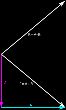
We can separate the incident vector I into two vectors, A and B (see figure) such that I = A + B. The reflection vector R is then equal to A - B.
I = A + B
R = A - B
We can compute B quite easily - it’s the projection of I onto the surface normal, or the dot product of I and N multiplied by N.
B = (I.N)N
Substitute that into both equations:
I = A + (I.N)N
R = A - (I.N)N
Then solve the first equation for A:
A = I - (I.N)N
And substitute into the second equation:
R = I - (I.N)N - (I.N)N
R = I - 2(I.N)N
We also adjust the origin slightly along the surface normal to avoid the same floating-point precision problems we had with our shadows earlier.
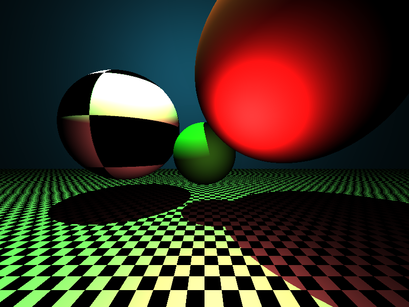
 Click to see high-resolution image. Note the recursive reflections between the
center sphere and the floor.
Click to see high-resolution image. Note the recursive reflections between the
center sphere and the floor.
Refraction
Refraction is again conceptually simple in a raytracer - trace a secondary ray (called the transmission ray) through the object in the appropriate direction and mix it in with the color of the object. Unfortunately, the math to construct the transmission ray is a lot more complex than it is to construct the reflection ray. But first, some definitions:
The transparency is the same as the reflectivity from before - the fraction of the final color that comes from refraction. Refraction is governed by a parameter called the index of refraction. When a ray of light passes from one transparent substance to another, it bends at an angle described by Snell’s Law:

sin(theta_i)/sin(theta_t) = eta_t/eta_i
Where theta_i and theta_t are the angle of incidence and angle of transmission, and eta_i and eta_t are the indices of refraction for the incident substance and the transmitting substance. We could calculate the angle of transmission using this equation, but we’ll need to do more to convert that angle into a vector.
As with reflection, refraction is really a two-dimensional process in the plane formed by the incident vector and the surface normal. This means that we can think of our transmitted ray as having a horizontal component (A) and vertical component (B). B is relatively simple to calculate:
B = cos(theta_t) * -N
This makes some intuitive sense - the transmitted ray will be on the opposite side of the surface from the incident ray, so it’s vertical component will be some fraction of the inverse of the surface normal. We use the cosine of the transmission angle because that’s how you calculate the vertical distance.
We can use this same approach to get the horizontal component A, but first we need to construct a horizontal unit vector (M). To do this, we first take the incident vector and subtract it’s vertical component, leaving only the horizontal component. We can calculate the vertical component of I easily - it’s (I.N)N, just like before. Then we normalize this horizontal vector to get the horizontal unit vector we need. We can slightly cheat here, though - the length of the horizontal component of I will be equal to sin(theta_i), so we can normalize using that instead of computing the vector length the slow way.
M = (I - -N(I.N)) / sin(theta_i) = (I + N(I.N)) / sin(theta_i)
A = sin(theta_t) * M
B = cos(theta_t) * -N
Putting this all back together, we get:
T = A + B
T = (sin(theta_t) * M) - N * cos(theta_t)
T = (sin(theta_t) * (I + N(I.N)) / sin(theta_i)) - N * cos(theta_t)
We can use Snell’s Law to replace that sin(theta_t) / sin(theta_i) with eta_i/eta_t, like so:
T = (I + N(I.N)) * eta_i/eta_t - N * cos(theta_t)
We could calculate cos(theta_t) from Snell’s Law and theta_i, but this involves lots of trigonometry, and ain’t nobody got time for that. Instead, we can express that in terms of a dot-product. We know from trigonometry that:
cos^2(theta_t) + sin^2(theta_t) = 1
cos(theta_t) = sqrt(1 - sin^2(theta_t))
And from Snell’s Law we know that:
sin(theta_t) = (eta_i/eta_t) * sin(theta_i)
Therefore:
cos(theta_t) = sqrt( 1 - (eta_i/eta_t)^2 * sin^2(theta_1) )
Then we can use the same trigonometric identity from above to convert that sin to a cosine:
cos(theta_t) = sqrt( 1 - (eta_i/eta_t)^2 * (1 - cos^2(theta_i)) )
And since cos(theta_i) = I.N, we get:
cos(theta_t) = sqrt( 1 - (eta_i/eta_t)^2 * (1 - I.N^2) )
And so, finally, we arrive at this monster of an equation (but look, no trigonometry):
T = (I + N(I.N)) * eta_i/eta_t - N * sqrt( 1 - (eta_i/eta_t)^2 * (1 - I.N^2) )
Now, there are a couple of wrinkles left to sort out. First, sometimes our ray will be leaving the transparent object rather than entering it. This is easy enough to handle, just invert the normal and swap the indices of refraction. We also need to handle total internal reflection. In some cases, if the angle of incidence is shallow enough, the refracted light ray actually reflects off the surface instead of passing through and travels back into the object. We can detect this when the term inside the sqrt is negative. Again, this makes intuitive sense - if that’s negative, the vertical component of the transmission vector would be positive (remember, B is a multiple of -N) and therefore on the same side of the surface as the incident vector. In fact, however, we can handle this by completely ignoring it, and I’ll explain why later.
Whew! Now that we have that giant equation, we can implement it in code, like so:
I also discovered a nasty bug in my sphere-intersection code while testing this. If you’re following along at home, this could be a good opportunity to practice your debugging. Go ahead, I’ll wait.
Hint: What happens if the ray origin is inside the sphere?
Find it? It turns out that the sphere-intersection test will return a point behind the origin of the ray if the origin is inside the sphere. The refraction ray will then intersect the sphere again, creating another refraction ray and so on until we hit the recursion limit. This took hours of painful debugging to find because I was looking for bugs in the create_transmission function. I didn’t realize that it was something else until I tried to create a refractive plane and noticed that it appeared to behave correctly.
Anyway, here’s the corrected sphere-intersection function:
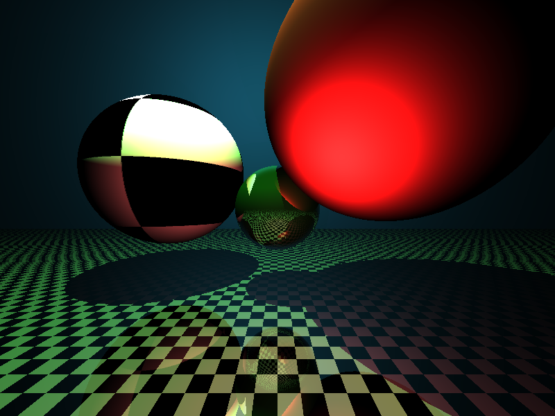
 Click to see high-resolution image. Notice the refracted image of the floor in
the transparent sphere.
Click to see high-resolution image. Notice the refracted image of the floor in
the transparent sphere.
Fresnel
However, we’re not quite done yet. If you’ve ever noticed how glass buildings or smooth lakes look like mirrors far away but clear up close, you know that transparent surfaces reflect light as well as transmitting it. It’s often even possible to see this effect in the polished floors of long hallways. These reflections are governed by the Fresnel Equations and we’ll have to simulate them to render refractive objects more accurately. Incidentally, this is why we can ignore total internal reflection in our transmission code above - the Fresnel code will cover that for us. We already know how to handle reflection in our code, but we need to calculate how much of a ray’s color comes from the refraction and how much from the reflection.
The derivation of the Fresnel Equations is hairy enough that Scratchapixel doesn’t even try to explain it. Serious physics-lovers might want to check out this derivation (PDF), but this is getting out of my depth so I’ll just take the final equations as given.
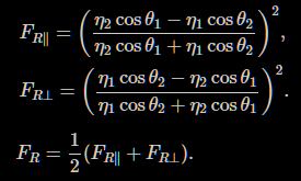
Fortunately for me, Scratchapixel does include some C++ code implementing these equations that I can simply translate to Rust:
And now that we have that, we can put it all together:
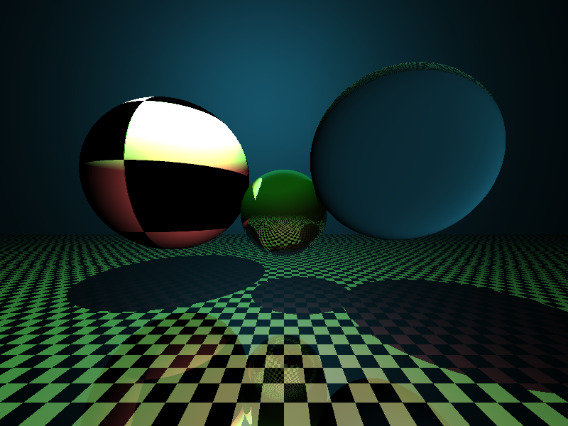
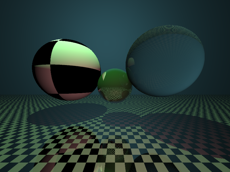
 Click to see high-resolution image
Beautiful, isn’t it?
Addendum - Gamma Correction
After I posted this article, fstirlitz pointed out that the lighting was a bit off because my code wasn’t handling Gamma Correction correctly (or at all). I had noticed the strange lighting effects but had simply assumed they were an artifact of my relatively simple rendering process, and that a more advanced renderer would solve them.
I’ll spare you a detailed discussion of what Gamma Correction is (if you’re interested, see What Every Coder Should Know About Gamma by John Novak). The short version is that human perception of light is non-linear. Our screens account for that by applying a power-law formula to the pixel values before displaying them. Correspondingly, image formats expect the pixel values to be in this non-linear color space, where my raytracer was writing out pixels in a linear color space. Likewise, when reading textures, it was reading non-linear color values and treating them as if they were linear. This mismatch caused the image to be generally darker, with sharper divisions between light and dark shades than the human eye would have seen.
Fortunately, this is pretty easy to fix:
I’ve only implemented the basic power-law formula rather than the more complex sRGB conversion, but it’s good enough for now.
 Click to see high-resolution image
Conclusion
This is the end of my series on raytracing, at least for now. There are many, many things I didn’t even begin to cover here. For instance, you might notice how the two lights in this scene don’t glint off the reflective objects the way real lights would, and how the glass sphere on the right doesn’t focus light rays on the floor like real glass would. If you’re interested, I encourage you to dig deeper - I may return to this subject myself in the future. Until then, I hope you’ve enjoyed reading.
As before, if you want to try playing around with the code yourself, you can check out the GitHub Repository.
Edit from the future: You may be interested in my next series on Writing a GPU-accelerated Path Tracer in Rust.