Writing a GPU-Accelerated Path Tracer in Rust - Part 3

Hello! Welcome to my third and final post on my GPU-accelerated Path Tracer in Rust. In the last post, we implemented all of the logic necessary to build a true path tracer. Problem is, even on the GPU it’s terrifically slow. This post is (mostly) about fixing that.

But first, we need to fix a bug or two, because I goofed. *sad trombone*

Step -1: Fixing Bugs

/u/anderslanglands on Reddit pointed out that, since I’m using Cosine-weighted Importance Sampling, I need to do some extra math to avoid biasing the results.

I’ll try to explain this as best I can, though I’m not totally sure I understand it myself. I think it works something like this: Monte-Carlo Integration isn’t just about taking the average of all of the samples. You have to weight each sample based on how likely it is for that sample to be chosen. In this case, that means how likely it is for each direction to be chosen. If we were choosing directions uniformly, then we could ignore this (because each sample would be equally likely and therefore every sample would have the same weight) but Cosine-weighted Importance Sampling means that we’re more likely to choose directions with a higher elevation than with a lower one. To correct for this, we need to calculate and return an additional weighting factor in create_scatter_direction. This is something I will definitely have to learn more about for future raytracing projects.

According to /u/anderslanglands, the weight is equal to the reciprocal of the dot product between the scatter direction and the surface normal. That’s easy enough to calculate:

And then in get_radiance we multiply the reflected_color against the returned weight:

let reflected_color = color
    .mul_s(cosine_angle)
    .mul_s(reflected_power)
    .mul_s(weight);

Conveniently, fixing this bug makes the scene bright enough that I can get away with removing an annoying hack where I multiplied all of the light values by a fudge factor. Hurray for correctness!

Now that the path tracer code works, it’s time to make it fast.

Step 0: Computing the Normal On-Demand

First, I’ll set up a scene that I can time without waiting for hours. By turning down the number of rays per pixel, the number of polygons, and the size of the image, I set up a scene that I can trace in about 45 seconds.

I had initially written the code to compute the polygon normals on the CPU and store them in the polygon structure. This costs 12 bytes per polygon, and three memory fetches each time we need the normal. Later on, I decided that this wasn’t a good compute/memory tradeoff, and changed the code so that the ray-triangle intersection test would calculate and return the normal as well. I didn’t expect this to make it much faster, but it did - rendering time for my test scene dropped to 35 seconds.

I’d expected a performance improvement, but I didn’t expect it to be so large. It avoids six memory fetches, or maybe only 3 is the compiler is smart enough, but I had thought that it was running enough threads at a time to hide the latency of the memory fetches. Perhaps I was incorrect.

The other performance improvement comes from packing the polygons closer together in memory. I haven’t written much about GPU performance concerns yet in this series, so I guess I’ll start here by explaining memory coalescing. You see, GPU’s don’t do caching like CPU’s do.¹ When a CPU instruction needs to read memory, the CPU will typically fetch many bytes (say, 128) following the area that it actually needs, and store them in a fast, on-chip memory space known as the cache. When the CPU then needs to read the next byte of memory, it doesn’t need to send a request all the way to main memory; it can fetch the result right out of the cache.

GPU’s instead do something called memory coalescing. When a GPU instruction needs to read memory, the GPU will fetch a block of memory, just like a CPU does (except even larger, like 1024 bytes). It will then pause the thread that requested it and process other threads in the meantime. Those other threads might make their own requests for memory, and it’s common for the other threads to request a location in memory that is in the same block of memory. When that block comes back, the GPU can wake up all threads waiting for the data it contains. This is called memory coalescing. Unlike the CPU, however, the GPU does not cache the returned block; if all of those threads then make another request for the next byte, that requires a second complete round-trip to memory.

Because of this, it’s beneficial when programming a GPU to arrange your memory and threads such that many threads’ requests can be satisfied with each memory fetch. Another way of thinking of it is that you should maximize the percentage of each fetch that will actually be used by a thread - if a single thread fetches one byte, that’s 1023 bytes that were loaded from memory and then discarded, and that’s inefficient.

I think this explains the speedup seen from calculating the normals on-demand rather than storing them in memory; the computation time of the calculation is small compared to the latency of the memory fetches, and meanwhile it makes all other memory fetches more efficient by packing the polygons closer together.

Step 1: Moller-Trumbore

Having already done some profiling, I know that the majority of the time is spent evaluating ray-triangle intersections. The intersection algorithm described earlier is not the most efficient possible algorithm, it’s just the only one that I was able to understand well enough to explain.

Frankly, I have no idea how the Moller-Trumbore intersection algorithm works, but I’m going to try it anyway. I don’t think it’s the fastest possible algorithm either, but it should be at least a bit faster. If your math-fu is stronger than mine, you can find Scratchapixel’s explanation here.

Once again, I was surprised at the magnitude of the change - this reduced the rendering time to just 15 seconds. And once again I’m puzzled as to why. It requires the same number of memory fetches. The computation is reduced somewhat, and this code is (or at least was) compute-bound, but I’m surprised that it would make it more than 50% faster. My best guess is that it allows more intersection tests to return early and skip much of the computation. In particular, it only computes the normal if the ray does intersect, where in the previous code it needed to compute the normal at the start of every test.

After some profiling, however, it appears that there is another factor at work. With this intersection-test code, the compiler has chosen to generate a kernel that uses fewer registers - few enough that the GPU can execute twice as many threads in parallel. This explains the majority of the speed increase.

Step 2: Structure-of-Arrays

Up until now, I’ve been using a simple polygon structure:

pub struct Polygon {
    pub vertices: [Vector3; 3],
    pub material_idx: usize,
}

My polygons are just collected together in a big array of polygon structures. That means that, for example, when a bunch of threads attempt to access the X coordinates of the first vertex in the first 32 polygons, each one is 44 bytes apart. As I discussed earlier, that means that every memory transaction will fetch a lot of bytes that ultimately end up discarded. A more efficient layout would have the X coordinates of the first vertices all together in one array, and then the Y coordinates in a second array, and so on.

However, I tried implementing this and it actually made the code go slower - two times slower, in fact. It appears as if this change caused the compiler to no longer be able to fit the kernel into 64 registers, and thus once again halved the number of concurrent threads. I’m going to keep these changes in a branch though; perhaps later changes will cause the register count to increase again, at which point this should become beneficial once more.

Step 3: Bounding Volumes

Although I can’t easily profile at the level of individual functions, I know from my last raytracer that ray intersection tests typically take up the large majority of time, especially for simple renderers like this. Right now, the path tracer traces every ray against every polygon. If you think about it, though, each ray will only ever pass through a small number of polygons; it would be better if we could build a data structure that would allow us to skip testing for intersections against polygons that won’t succeed.

There are many such data structures available. I’m going to go with one of the simpler ones, but before that, there’s some work to do first.

First up, I’ll add more polygons to the scene to bring the rendering time back up. Second, I’ll add some statistics measurement so we can see how many intersection tests are actually being performed:

18984 polygons in scene
Trace time: 91692.906250ms
Traced 27072102 rays
Performed 513936784368 triangle intersections

Well, look at that. 27 million rays and over half a trillion intersection tests done in a minute and a half (and with not-very-optimized code). GPUs are pretty great.

Incidentally, just adding the statistics counting broke whatever spell had caused the compiler to use fewer registers, so I tried using my structure-of-arrays changes from earlier, and that actually made it slower. Go figure.

One way to reduce the number of intersection tests is to first test each ray against some kind of bounding volume; a simple shape that is cheap to test against, but which contains many polygons (eg. all polygons for an object). If a ray doesn’t intersect the bounding volume, we know that it won’t intersect any of the polygons it contains, so we can skip testing those polygons.

In this case, I’ll go with an axis-aligned bounding box because those are easy to construct - just loop over all vertices of all polygons in an object and track the min/max x, y, and z coordinates. These become the bounds of our bounding box. The down-side of using a bounding box is that there are a lot of rays that will intersect with the box that don’t actually intersect any of the polygons, but that’s the price we pay for simplicity.

Now that we have a bounding box for each object, we need to be able to test rays against it. I’ll start in two dimensions and then generalize to three.

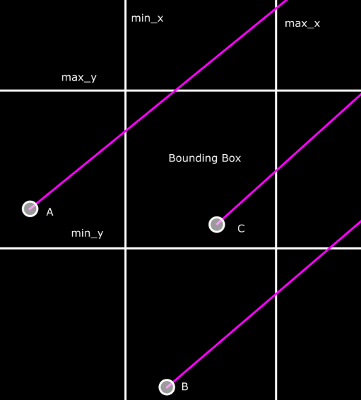
From geometry, we know that the equation of a line is y = mx + b. We can use this to calculate the y coordinate at the point where the ray intersects with an axis-aligned plane. Consider ray A in the image above. It intersects the line at min_x. We can calculate the y coordinate of that intersection by substituting into that line equation - y = A.direction.y * (min_x - A.origin.x) + A.origin.y. From there, we could test if the min_y <= y <= max_y, and if so, there’s an intersection. If not, we’d repeat for the other three sides of the box.

However, this is slower than it needs to be, especially in 3D. With three dimensions, you’d have to check if the y and the z values are in the right ranges for a total of four comparisons times six sides, as well as the calculations to find the intersection points. Instead, take another look at the image, specifically ray B. Notice that the distance to the min_y plane is greater than the distance to the max_x plane? This makes it possible to use a faster test. Specifically, if the distance to min_x is greater than the distance to max_y or if the distance to min_y is greater than the distance to max_x, the ray will miss the bounding box. Note that if the ray direction is something other than up-and-right, we might have to swap the different planes around a bit. This test even works if the ray origin is inside the bounding box, like ray C. For that ray, the distance to min_x and min_y will be negative, and therefore always less than the distance to max_y or max_x, so the test will always detect an intersection. If you like, take some time thinking through various scenarios and convince yourself that this works. ²

18984 polygons in scene
Trace time: 54580.031250ms
Traced 27073011 rays
Performed 135365055 bounding-box intersections
Performed 73669018592 triangle intersections

From 90 seconds down to 55 seconds, and the number of triangle intersections is down to 73 billion - just 14% of what it was previously, at the cost of a hundred million or so bounding-box tests. Much better!

Step 4 - Grid Marching

I’m not finished yet, though. Even if a ray hits the bounding box, it will still only intersect a small number of the polygons contained within. Now that we can skip objects that can’t intersect with a ray, it would be nice if we could likewise skip polygons within an object that can’t intersect.

For once, I’m going to deviate from Scratchapixel here and do something different. I’m going to use the algorithm proposed in A Fast Voxel Traversal Algorithm for Ray Tracing by Amanatides and Woo. The reason I picked this algorithm is because I’m already familiar with it. You see, years ago I spent some time writing a mod for Minecraft which added a variety of customizable ray-guns and blasters to the game. I never did end up releasing it or anything (though the code is on my GitHub if you’re really curious), but one of the things I needed while working on it was a fast way to trace a ray from the player’s blaster through the blocky world of Minecraft. There was a built-in ray test function, but it could only return the first intersection with a block and (since some of the rayguns could shoot through blocks) I needed an alternate test that could produce a list of all blocks hit. In the end, I ended up modifying Amanatides and Woo’s algorithm, so I thought it fitting that I should use it again for its intended purpose of raytracing.

This algorithm works by dividing the scene (or, in my case, the object) into a 3D grid of boxes called voxels. To trace a ray agaist an object, we determine the point at which the ray enters the grid and some information about its direction, then step across the grid, testing the ray against all polygons in the current voxel - ignoring all polygons that aren’t in one of the voxels the ray passes through. This requires some extra local variables:

let t_max_x, t_max_y, t_max_z;
let t_delta_x, t_delta_y, t_delta_z;
let step_x, step_y, step_z;
let cur_x, cur_y, cur_z;

These require some explanation. t_delta_x represents how many units we must move along the ray such that the X component of that movement is equal to the width of a voxel in the X direction, and the same goes for the other deltas. t_max_x represents how many units away along the ray from the ray origin we would have to move to enter the next voxel in the X direction, and likewise the same goes for the other max values. The step variables hold positive or negative one, depending on the sign of the ray direction in that axis. As you might expect, cur_x simply holds the number for the current voxel in the X direction.

The loop proceeds like this. First, we find which axis has the closest boundary to the next voxel - that is, the minimum of t_max_x, t_max_y, t_max_z. If, for example, t_max_y is the smallest, that means that the ray will pass into the next voxel in the Y direction first. Then, we step one voxel in that direction (add step_y to cur_y), update the appropriate maximum (The next Y-axis voxel boundary is t_delta_y units away, so add that to t_max_y), and test the polygons in the new voxel. That’s it!

Well, not quite. Some polygons will be in multiple voxels, and this creates an odd corner case that we need to deal with first.

Image: voxel_marching_corner_case

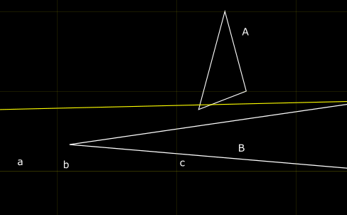
Consider the ray (yellow line) in this image. It first enters the voxel b and traces against polygon B - and indeed, it does intersect. If we stopped there, we would never notice that there is a closer intersection with polygon A in voxel c. We can handle this by checking the returned intersection distance to B - it will be greater than the minimum of t_max_x, t_max_y, t_max_z, so we know that that intersection is not in this voxel and we can ignore it until we actually reach the voxel containing the intersection. This does mean that we might perform an intersection test against the same polygon multiple times, but that’s an acceptable price to pay for skipping all of the other polygons.

There are still a few things left to do, however. How do we construct the grid? How do we determine how many boxes there should be in the grid?

There is no algorithm for determining the optimal grid size, but we can come up with something fairly good using the following equation:

n_x = d_x * cube_root((fudge_factor * num_polygons) / bounding_box_volume)

n_x is the number of grid cells in the x direction, and d_x is the size of the grid in the x direction. The fudge factor is just a user-defined parameter to adjust the grid size, and the rest are self-explanatory. I’ll go with a fudge factor of 4.0 because that seems like a nice, round number. We can trivially apply the same formula to the other two axes as well. As for constructing the grid, we can take the bounding box of each polygon and insert it into every grid cell that intersects that bounding box. This is easy to implement, but it does mean that some polygons will be added to grid cells that they aren’t actually in. Once again, we’ll just ignore this.

With all of that implemented, here’s the new stats:

18984 polygons in scene
Trace time: 21850.224609ms
Traced 88874605 rays
Performed 444373025 bounding-box intersections
Performed 3181122057 triangle intersections

I’ve changed some settings in the meantime, so this isn’t quite a fair comparison. Note that the number of rays has gone way up to 89 million (previously 27 million), but despite that we’re down to 3 billion triangle intersections (from 73 billion) and 20 seconds (from 55). That’s pretty respectable!

Conclusion

These improvements don’t just make the renderer faster; they also increase the complexity of the scenes that we can render in a reasonable time. Such as the beautiful image below:

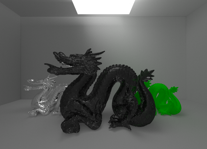
Click for full size.

Here’s the stats for this one:

300024 polygons in scene
Trace time: 49543072.000000ms
Traced 118162718847 rays
Performed 590813594235 bounding-box intersections
Performed 8472990410182 triangle intersections

That works out to almost 14 hours. There’s still a lot of room for improvement, but I’m pretty happy with that.

I think I’m done with this particular project, at least for now. I’ve had a lot of fun learning about GPU programming, even if it isn’t always the easiest thing to do in Rust.

There’s a few things that I would consider for future renderers, if I ever decide to write one. First, my understanding of the math and the algorithms is largely based on whatever I could cobble together from online sources, so I’d probably want to have a better understanding before doing a third renderer. I’ve heard that Physically Based Rendering by Pharr et. al. is a good resource for this. Second, I probably wouldn’t try to use path tracing and nothing else, like I did here. More sophisticated algorithms (or even basic ones like tracing both shadow rays and scattered paths) produce a much nicer image with far fewer rays than using path-tracing to do all of the lighting. Third, I’m not sure about the design of my kernel code. I put everything into one giant kernel function, but this led to recurring problems with register pressure and code complexity. If I were doing it again, I would consider structuring it as a Wavefront Path Tracer instead.

That’s just about it from me. I hope you’ve enjoyed reading, and as always, you can check out the code on GitHub.