Hello! This is part one of a short series of posts on writing a simple raytracer in Rust. I’ve never written one of these before, so it should be a learning experience all around.
So what is a raytracer anyway? The short version is it’s a computer program that traces the paths of simulated rays of light through a scene to produce high-quality 3D-rendered images. Despite that, it also happens to be the simplest way to render 3D images. Unfortunately, that comes at a cost in render time - raytracing an image takes much longer than the polygon-based rendering done by most game engines. This means that raytracing is typically used to produce beautiful still images or pre-rendered video (eg. Pixar’s RenderMan technology).
For the purposes of this post, I’ll assume that you’re familiar with what vectors are and how they work, as well as basic geometry. If you aren’t, check out the first three pages of Scratchapixel’s excellent series on geometry and linear algebra. You don’t need to know Rust specifically (though I recommend it, it’s a great language) but you should at least be familiar with C-family programming languages. If you want to build the code however, you will need to install Cargo, which is the standard Rust build tool.
Defining the Scene
The first thing to do is decide exactly what our scene (and therefore our renderer) will be able to handle. For this first post, it won’t be much. One lonely sphere, hanging in the darkness. No lighting, reflection, or transparency. No other shapes. We’ll extend this basic scene over the rest of this series.
We’ll start by defining some structures to hold our scene data:
And a stub render method and simple test case. I’m using the image crate to set up the image buffer and write the resulting render to a PNG file. This is all pretty straightforward except for the position of the sphere - (0.0, 0.0, -5.0). I’ll explain that later.
Prime Ray Generation
The basic idea of how a raytracer like this works is that we iterate over every pixel in the finished image, then trace a ray from the camera out through that pixel to see what it hits. This is the exact opposite of how real light works, but it amounts to pretty much the same thing in the end. Rays traced from the camera are known as prime rays or camera rays. There is actually a lot of freedom in how we translate pixel coordinates to prime rays, which confused me for a while, but it’s pretty simple if you follow common conventions.
We’ll start with defining a Ray structure and a static function for generating prime rays:
By convention, the camera is aligned along the negative z-axis, with positive x towards the right and positive y being up. That’s why the sphere is at (0.0, 0.0, -5.0) - it’s directly centered, five units away from the camera. We’ll start by pretending there’s a two-unit by two-unit square one unit in front of the camera. This square represents the image sensor or film of our camera. Then we’ll divide that sensor square into pixels, and use the directions to each pixel as our rays. We need to translate the (0…800, 0…600) coordinates of our pixels to the (-1.0…1.0, -1.0…1.0) coordinates of the sensor. I’ll start with the finished code for this step, then explain it in more detail.
Let’s unpack that a bit and focus on only the x component. The y component is almost exactly the same.
let pixel_center = x as f64 + 0.5;
let normalized_to_width = pixel_center / screen.width as f64;
let adjusted_screen_pos = (normalized_to_width * 2.0) - 1.0;
First, we cast to float and add 0.5 (one half-pixel) because we want our ray to pass through the center (rather than the corner) of the pixel on our imaginary sensor. Then we divide by the image width to convert from our original coordinates (0…800) to (0.0…1.0). That’s almost, but not quite, the (-1.0…1.0) coordinates we want, so we multiply by two and subtract one. That’s all there is to it! The y calculation follows the same basic process except the last step:
let adjusted_screen_pos = 1.0 - (normalized_to_width * 2.0);
This is simply because the image coordinates have positive y meaning down, where we want positive y to be up. To correct for this, we simply take the negative of the last step of the calculation.
Then we pack the x and y components into a vector (z is -1.0 because all of our prime rays should go forward from the camera) and normalize it to get a nice direction vector. Simple, right? This is why the 2x2 sensor 1 unit from the camera convention is convenient. If we’d used any other set of coordinates than (-1.0…1.0, -1.0…1.0) then the image would be off center and/or we’d have to do more calculations to avoid distorting it.
We could actually stop here - this is a working prime ray generation function. However, it assumes that the image we’re generating is perfectly square and that the field of view is precisely 90 degrees. It’s probably worth adding a correction for other aspect ratios and different fields of view.
To adjust for different aspect ratios, we calculate the aspect ratio and multiply it by the x coordinate. We’re assuming that the image will be wider than it is tall, but most images are so that’s good enough for now. If we didn’t do this, the rays would be closer together in the x direction than in the y, which would cause a distortion in the image (where every pixel is the same size in both directions).
Then we can add another adjustment for field of view. Field of view is the angle between the left-most ray and the right-most ray (or top- and bottom-most). We can use simple trigonometry to calculate how much we need to adjust the coordinates by:
You might have noticed that the origin of all prime rays is exactly (0, 0, 0). This means that our camera is fixed at those coordinates. It is possible to adapt this function to place the camera in different locations or orientations, but we won’t need that for now.
Testing for Intersections With The Sphere
Now that we have our prime rays, we need to know if they intersect with our sphere. As usual, we’ll start with some definitions.
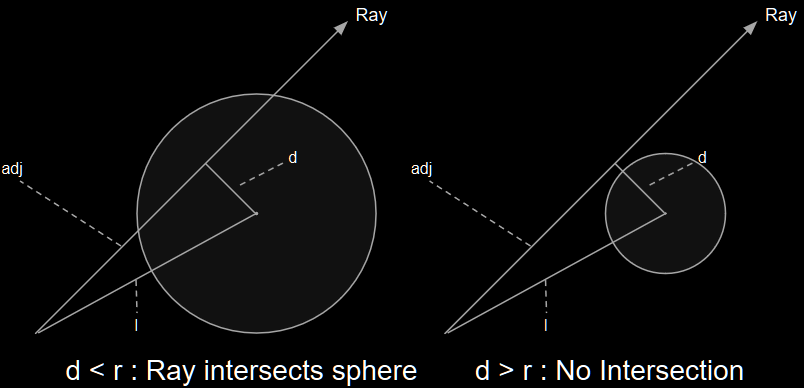
The basic idea behind this test is that we construct a right-triangle using the prime ray as the adjacent side and the line between the origin and the center of the sphere as the hypotenuse. Then we calculate the length of the opposite side using the Pythagorean Theorem - if that side is smaller than the radius of the sphere, the ray must intersect the sphere. In practice, we actually do the check on length-squared values because square roots are expensive to calculate, but it’s the same idea.

Finishing the Render Method
Now that we have all of the hard parts done, we simply need to integrate these functions into the render function and produce our image:
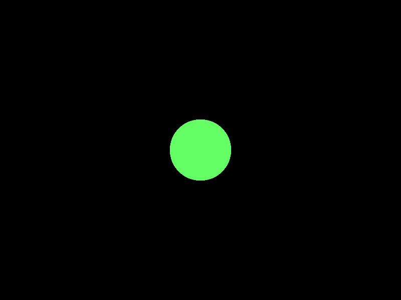
After adding some extra glue code to parse a scene definition and save the rendered image to a file, we get the resulting image:

It isn’t very impressive yet, but we’ll add more detail to it as we go. In the next post, we’ll add planes, multiple spheres, and some basic lighting effects.
If you want to try playing around with the code yourself, you can check out the GitHub Repository. If you want to learn more about 3D rendering in general or raytracing in particular, check out Scratchapixel, which is the resource I used while working on this.
Thanks to Scott Olson and Daniel Hogan for suggesting improvements to an earlier version of this article.